

RANDOM FOREST WITH US ADULT INCOME DATASET
-
date_range 08/03/2019 18:00 infosortMachine LearningRandom forestlabelDecision treesPruning
Random Forest
Random Forest is simply a collection of Decision Trees that have been generated using a random subset of data. In order to understand a Random Forest, you have to understand a Decision Tree.
Decision trees
The goal is to create a model that predicts the value of a target variable based on several input variables. A Decision tree is a flowchart like tree structure, where each internal node denotes a test on an attribute, each branch represents an outcome of the test, and each leaf node (terminal node) holds a class label. The topmost node in a tree is the root node. A tree can be “learned” by splitting the source set into subsets based on an attribute value test. This process is repeated on each derived subset in a recursive manner.
- Instances are represented by attribute-value pairs
- The target function has discrete output values
- Disjunctive descriptions may be required
- The training data may contain errors : Decision tree methods are robust to errors
- The training data may contain missing attribute values.
Decision tree learning has been applied to problems such as classify medical patients by their disease, equipment malfunctions by their cause and loan applicants by their likelihood of defaulting on payments.
In real data mining situations, the problem is that the decision tree constructed may become gigantic. So it becomes important to find techniques to minimize the size of the tree, as far as possible. The idea is to put the decision nodes which give the most information highest (closest to the root) in the decision tree.
Most algorithms used in decision tree learning algorithms are variations of ID3 algorithm.The ID3 algorithm can be summarized in the following way:
1- Calculate the entropy of every attribute using the data set
2- Split the set \(S\) into subsets using the attribute for which the resulting entropy (after splitting) is minimum (or, equivalently, information gain is maximum)
3- Make a decision tree node containing that attribute
4- Recurse on subsets using remaining attributes.
First we define a statistical property called, information gain that measures how well a given attribute separates the training examples according to their target classification. ID3 uses this information gain measure to select among the candidate attributes at each step while growing the tree.
In order to define information gain measure first we define entropy that characterizes the (im)purity of an collection of examples. Given a collection \(S\) containing positive and negative example of some target concept, the entropy of \(S\) relative to this boolean classification is:
\[Entropy\space(S) = -p_+log_2p_+ -p_{-}log_2p_-\]Where \(p_+\) is the proportion of positive example in \(S\) and \(p_{-}\) is the proportion of negative example in \(S\). To illustrate suppose \(S\) is a collection of 14 examples of some boolean concept ,including 9 positive and 5 negative The the entropy is calculated in the following way:
\[Entropy\space(S) = - \frac{9}{14}log_2(\frac{9}{14}) - \frac{5}{14}log_2(\frac{5}{14})\]Note the entropy is 1 when we have an equal quantity of negative and positive values. More generally, if the target attribute can take on c different values, then the entropy of \(S\) relative
Which attribute to select as the root?
| Windy | Outlook | Humidity | Temperature | Play golf? |
|---|---|---|---|---|
| Weak | sunny | high | hot | no |
| Strong | sunny | high | hot | no |
| Weak | overcast | high | hot | Yes |
| Weak | rain | normal | cool | Yes |
| Strong | overcast | normal | cool | Yes |
| Weak | sunny | hight | mild | no |
| Weak | sunny | normal | cool | Yes |
| Weak | rain | normal | mild | Yes |
| Strong | sunny | normal | mild | Yes |
| Strong | overcast | high | mild | Yes |
| Weak | overcast | normal | hot | Yes |
| Strong | rain | high | mild | no |
| Strong | rain | normal | cool | no |
| Weak | rain | high | mild | Yes |
Let’s calculate the entropy
- Outlook -> sunny: 3 examples yes, 2 examples no.
- Outlook -> overcast: 4 examples yes, 0 examples no
- Outlook->rainy : 2 examples yes, 3 examples no.
How can we compute the quality of the entire split?
Compute the weighted average over all sets resulting from the split weighted by their size.
\[I(S,A) = \sum_ {i} \frac{|S_i|}{|S|} E(S_i)\]Average entropy for attribute Outlook:
\[I(Outlook)=\frac{5}{14}⋅0.971+ \frac{4}{14}.0 +\frac{5}{14}⋅0.971=0.693\]When an attribute \(A\) splits the set \(S\) into subsets \(S_i\)
- we compute the average entropy
- and compare the sum to the entropy of the original set \(S\)
Information Gain for Attribute A
\[Gain(S,A) = E(S)- I(S,A) = E(S)- \sum_ {i} \frac{|S_i|}{|S|} E(S_i)\]The attribute that maximizes the difference is selected:
Maximizing information gain is equivalent to minimizing average entropy, because \(E(S)\) is constant for all attributes A.
Entropy:
- Humidity -> High: 3 examples ‘Yes’, 4 examples ‘No’
- Humidity -> Normal: 6 examples ‘Yes’, 1 example ‘No’
- Wind ->Weak: 6 examples ‘Yes’, 2 examples ‘No’
- Wind ->Strong :3 examples ‘yes’, 3 examples ‘No’
- Temperature -> Hot : 2 examples ‘No’, 2 example ‘Yes’
- Temperature-> Cool: 3 examples ‘Yes’, 1 examples ‘No’
- Temperature-> Mild: 4 examples ‘Yes’, 2 ‘No’
- The set:
Information Gain
\[Gain (S, Humidity) = 0.940- \frac{7}{14}0.985 - \frac{7}{14}0.592 = 0.151\] \[Gain (S, Outlook) = 0.940- \frac{7}{14}0.985 - \frac{7}{14}0.592 = 0.246\] \[Gain (S, Wind) = 0.940- \frac{7}{14}0.811 - \frac{7}{14}1 = 0.048\] \[Gain (S, Temperature) = 0.940- \frac{4}{14}1 - \frac{4}{14}0.8112 - \frac{6}{14}0.9182 = 0.029\]Outlook has the highest value, so it is selected as the root node.
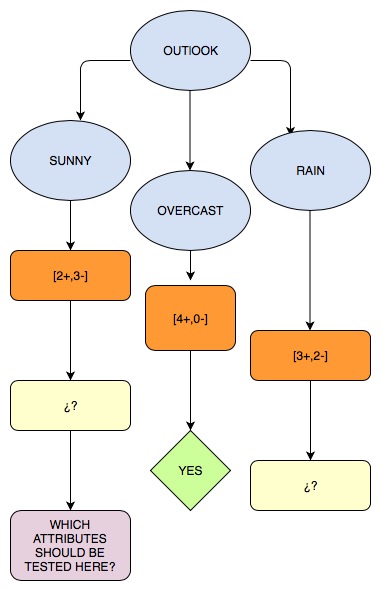
Entropy
- Humidity -> High : 3 examples sunny and all of them belongs to ‘No’ class
- Humidity -> Normal: 2 examples sunny and all of them are ‘Yes’
- Wind -> Weak: 3 examples sunny, 2 are ‘no’, and the other is ‘Yes’
- Wind -> Strong: 2 examples sunny, 1 is ‘yes’, and the other ‘no’
- Temperature -> Hot: 2 examples sunny and both ‘No’
- Temperature -> Mild: 2 examples sunny, 1 ‘No and 1 ‘Yes’.
- Temperature -> Cool: 1 examples sunny and belongs to ‘Yes’ class.
Information gain:
\[Gain(Sunny,Humidity) = 0.971 -\frac{3}{5}.0 - \frac{2}{5}0 = 0.971\] \[Gain (Sunny, Wind) = 0.971 -\frac{3}{5}0.9182 -\frac{2}{5}1.0 = 0.20\] \[Gain (Sunny, Temperature) = 0.971 -\frac{2}{5}.0 - \frac{1}{5}.0 - \frac{2}{5}.1 = 0.571\]We choose the biggest value, so Humidity is selected.
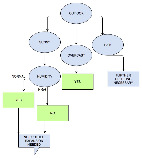
Then we do it all again for the two left attributes and we decide the attribute with the highest value.
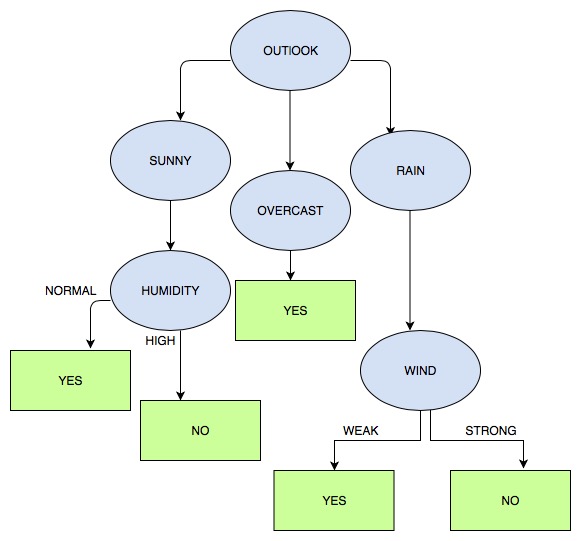
Final Decision tree
Issues in decision tree learning
Overfitting typically occurs when we try to model the data training perfectly.It might be due to insufficient examples. Overfitting results in decision trees that are more complex than necessary
How can we spot overfitting? Low training error and testing error is comparably high
Measures against overfitting or growing the tree too deep
Pre-Pruning : Stop growing the tree earlier, before it reaches the point where it perfectly classifies the training data.
Post-Puning :Allows the tree to overfit the data, and then post-prune the tree
In practice we usually use the second approach as it is easier to post-prune the data than estimating the time to stop growing the tree.
The important step of tree pruning is to define a criterion be used to determine the correct final tree size. We can use the following methods
- Use a validation set, to evaluate the effect of post-pruning nodes from the tree. Then we have a validation train to build a tree, a validation set to prune the tree and then the set to evaluate the model.
- Build the tree by using the training set, then apply a statistical test to estimate whether pruning or expanding a particular node is likely to produce an improvement beyond the training set. (E.g Chi-square test)
- Minimum Description Length Principle : Use an explicit measure of the complexity for encoding the training set and the decision tree, stopping growth of the tree when this encoding size (size(tree) + size(misclassifications(tree)) is minimized.
Rule Post-Pruning
1- Growing the tree until the training data is fit as well as possible and allowing overfitting.
2- Convert the learned tree into an equivalent set of rules by creating one rule for each path from the root node to the leaf node.
3- Prune each rule by removing any preconditions that result in improving its estimated accuracy.
4- Sort the pruned rules by estimated accuracy.
To illustrate this considerer the last diagram. Each attribute test along the path from the root to the leaf node becomes a rule antecedent (precondition) and the classification at the leaf node becomes the rule consequent (postcondition).
For example the leftmost path of the tree is translated into the rule : IF (OUTLOOK=SUNNY) ^ (HUMIDITY = NORMAL) THEN (PLAYTENNIS = YES)
Next each rule is pruned by removing any precondition whose removal doesn’t worsen its estimated accuracy. Given the above rule we will considerer to remove (OUTLOOK=SUNNY) and (HUMIDITY = NORMAL) and select whichever of this pruning steps improve estimated accuracy. No pruning step is performed if it reduces the estimated rule accuracy. So how do we measure this? One way is to use a validation set disjoint for the training set
Important Parameters to tune in Scikit Algorithm
1) N_ESTIMATORS: The more trees the less likely the algorithm is to overfit. The higher the number of trees the better to learn the data.
2) CRITERION: Here you can use Entropy or Gini criteria.
3) MAX_DEPTH : Gives limit on vertical depth decide up to which level pruning is required.
4) MIN SAMPLES SPLIT : Minimum number of samples required to split an internal node. High value: Underfitting, Low value: Overfitting
5) MIN SAMPLES LEAF: The branch will stop splitting once the leaves have that number of samples each.
6) MAX FEATURES: Represents the number of features to consider when looking for the best split The smaller, the less likely to overfit, but too small will start to introduce under fitting.
US Adult Income Dataset
Now let's put this into practice with us adult income salary . We are going to use random forest in order to predict whether an individual's salary is greater than 50 K or not.
- First we explore the data to understand the trends in the corpus.
- Then use this information to predict whether an -individual made more or less than $50,000
Each entry contains the following information about an individual:
- Age
- Work-class: Term to represent the employment status of an individual. Such as : Private, Localgov, Stategov, Withoutpay, Neverworked and so on
- Fnlwgt: Term to represent final weight.The number of units in the target population that the responding unit represents
- Education: the highest level of education achieved by an individual. Such as Bachelors, Somecollege, 11th, HSgrad, Profschool,9th, 7th8th, 12th, Masters, 1st4th, 10th and so on.
- Education num: the highest level of education achieved in numerical form
- Marital status: marital status of an individual. Such as Divorced, Never married, Separated, Widowed,
- Occupation: the general type of occupation of an individual Such as Techsupport, Craftrepair, Otherservice, Sales, Execmanagerial and so on
- Relationship: Represents the responding unit’s role in the family. Such as Wife, Husband and so on
- Race: Descriptions of an individual’s race Such as: White, AsianPacIslander, AmerIndianEskimo, Other, Black.
- Sex: the biological sex of the individual Such as :Male, Female
- Capital gain: capital gains for an individual
- Capital loss: capital loss for an individual
- Hours per week: the hours an individual has reported to work per week
- Native country: country of origin for an individual Such as UnitedStates, Cambodia, England, PuertoRico and so on
- Income: whether or not an individual makes more than $50,000 annually. ○ <=50k, >50k
import pandas as pd
import matplotlib.pyplot as plt
import seaborn as sns
from sklearn.preprocessing import Imputer
from sklearn import preprocessing
from sklearn.model_selection import train_test_split
from sklearn.metrics import confusion_matrix
from sklearn.ensemble import RandomForestClassifier
from sklearn.metrics import accuracy_score
dataset = 'https://archive.ics.uci.edu/ml/machine-learning-databases/adult/adult.data'
row_names = ["Age", "Workclass", "Fnlwgt", "Education", "EducationNum", "MaritalStatus",
        "Occupation", "Relationship", "Race", "Gender", "CapitalGain", "CapitalLoss",
        "HoursPerWeek", "Country", "Income"]
us_adult_income = pd.read_csv(dataset, names=row_names,na_values=[' ?'])
us_adult_income.describe()
| Age | Fnlwgt | EducationNum | CapitalGain | CapitalLoss | HoursPerWeek | |
|---|---|---|---|---|---|---|
| count | 32561.000 | 32561.000 | 32561.000 | 32561.000 | 32561.000 | 32561.000 |
| mean | 38.582 | 189778.367 | 10.081 | 1077.649 | 87.304 | 40.437 |
| std | 13.640 | 105549.978 | 2.573 | 7385.292 | 402.960 | 12.347 |
| min | 17.000 | 12285.000 | 1.000 | 0.000 | 0.000 | 1.000 |
| 25% | 28.000 | 117827.000 | 9.000 | 0.000 | 0.000 | 40.000 |
| 50% | 37.000 | 178356.000 | 10.000 | 0.000 | 0.000 | 40.000 |
| 75% | 48.000 | 237051.000 | 12.000 | 0.000 | 0.000 | 45.000 |
| max | 90.000 | 1484705.000 | 16.000 | 99999.000 | 4356.000 | 99.000 |
Distribution of educational attainment
plt.figure(figsize=(25,8))
sns.countplot(y='Education', data = us_adult_income, order = us_adult_income.Education.value_counts().index)
plt.title('Education')
plt.xlabel('Number of Occurrences', fontsize=12)
plt.ylabel('Degree', fontsize=12)
plt.show()
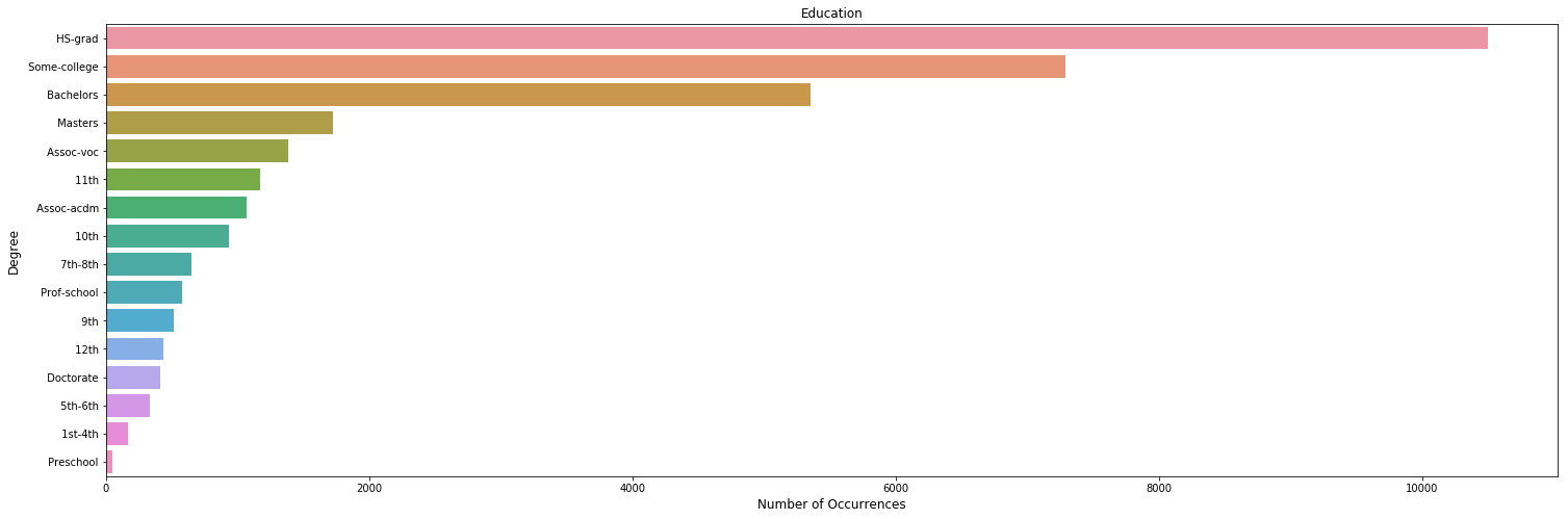
Most of the individuals in the dataset have at most a high school education, and have attended an University while only a small portion have a doctorate.
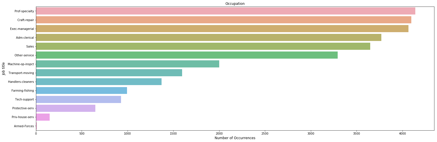
Job title Distribution
plt.figure(figsize=(25,8))
sns.countplot(y='Occupation',order= us_adult_income.Occupation.value_counts().index, alpha=0.8,data = us_adult_income)
plt.title('Occupation')
plt.xlabel('Number of Occurrences', fontsize=12)
plt.ylabel('Job title', fontsize=12)
plt.show()
Countries Distribution
plt.figure(figsize=(20,4))
sns.countplot(y='Country',order=us_adult_income.Country.value_counts().index[:10], alpha=0.8,data = us_adult_income)
plt.title('Countries')
plt.ylabel('Number of Occurrences', fontsize=12)
plt.xlabel('Countries', fontsize=12)
plt.show()
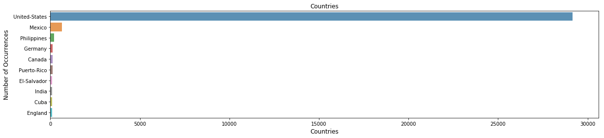
Most the people that have been surveyed are from US.
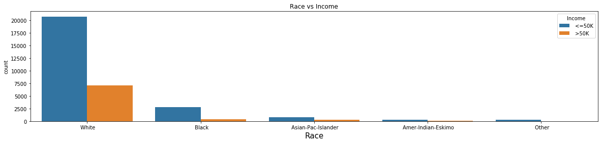
Race Distribution
plt.figure(figsize=(20,4))
plt.title('Race Distribution')
plt.ylabel('Race', fontsize=15)
sns.countplot(y = 'Race', data=us_adult_income)
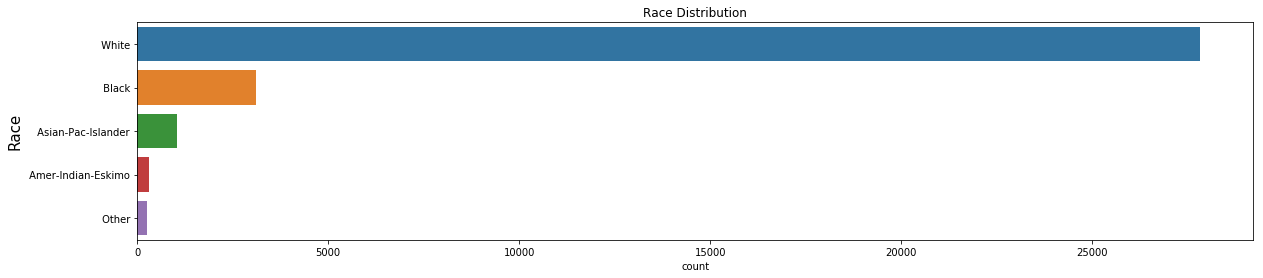
The sample size of Whites in the dataset is disproportionately large in comparison to all other races.
Gender vs Income
sns.barplot(x = 'Gender',y='Age' ,hue='Income', data=us_adult_income)
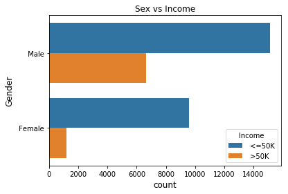
The percentage of males who make greater than $50,000 is much greater than the percentage of females that make the same amount.
Box plot for hours per week grouped by gender vs Income
sns.boxplot(x = 'Gender',y='HoursPerWeek' ,hue='Income', data=us_adult_income)
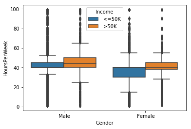
The median of hours per week for women is smaller than the one for men. The majority of people who perceive more than 50 K are men
Education vs Income
plt.figure(figsize=(25,10))
sns.countplot(x = 'Education',hue='Income', data=us_adult_income)
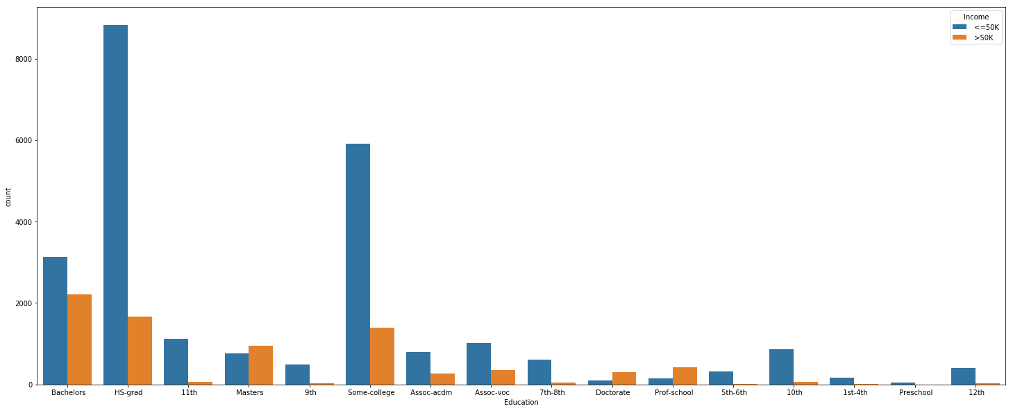
People who achieve a higher level of education tend to earn more than 50K
Occupation vs Income
plt.figure(figsize=(25,10))
sns.countplot(x = 'Occupation',hue='Income', data=us_adult_income)
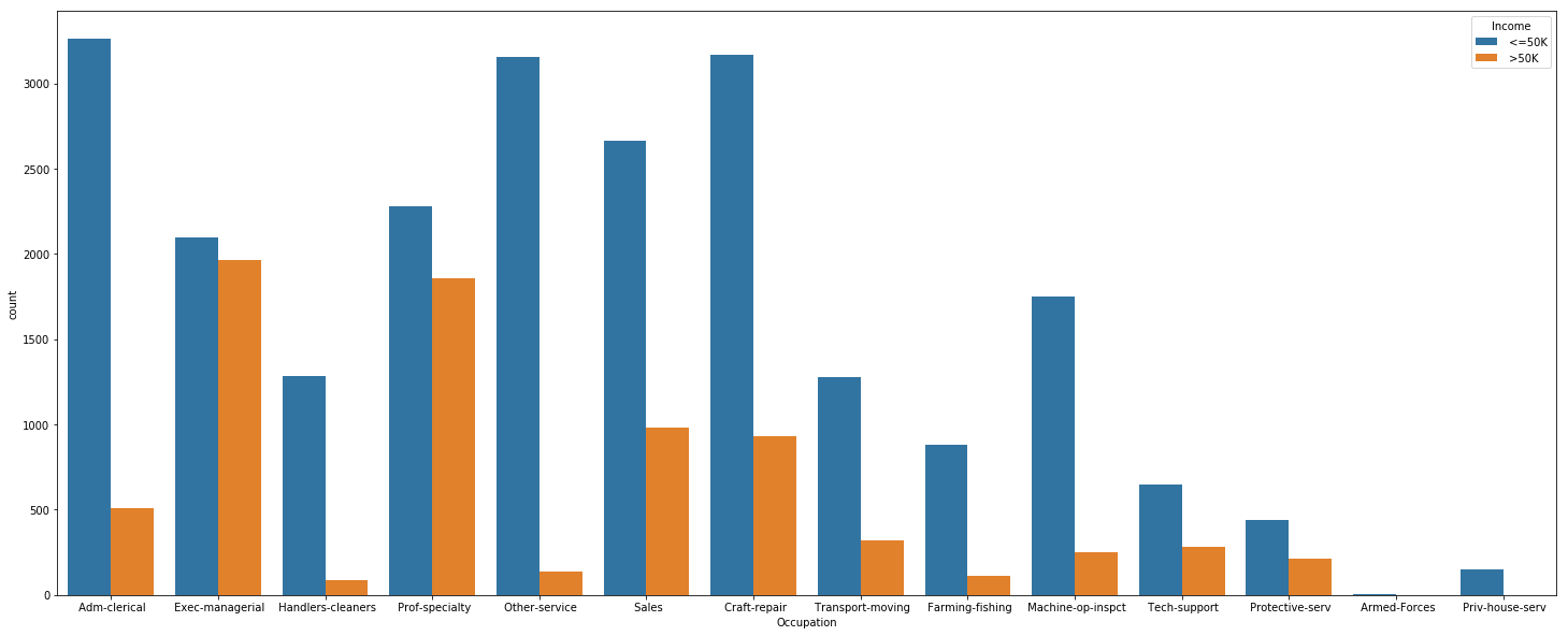
Exec-managerial and Prof-specialty stand out as having very high percentages of individuals making over $50,000. In addition, Priv-House-Serv make only less than 50 K
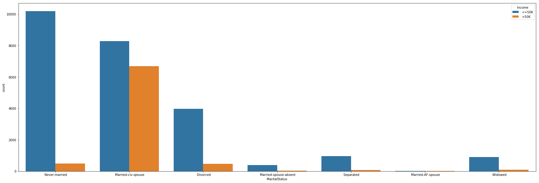
Marital Status vs Income
plt.figure(figsize=(30,10))
sns.countplot(x = 'MaritalStatus',hue='Income', data=us_adult_income)
Work-class vs Income
plt.figure(figsize=(20,10))
sns.countplot(x = 'Workclass',hue='Income', data=us_adult_income)
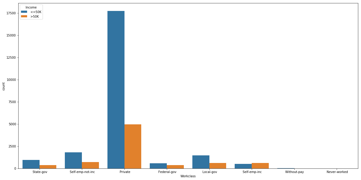
Federal-gov and self-emp-inc are the the two classes which almost equal in people who make more than 50K and less.
Age vs Income
plt.figure(figsize=(20,10))
plt.title('Age vs Income')
plt.xlabel('Age', fontsize=15)
sns.countplot(x = 'Age',hue='Income', data=us_adult_income)
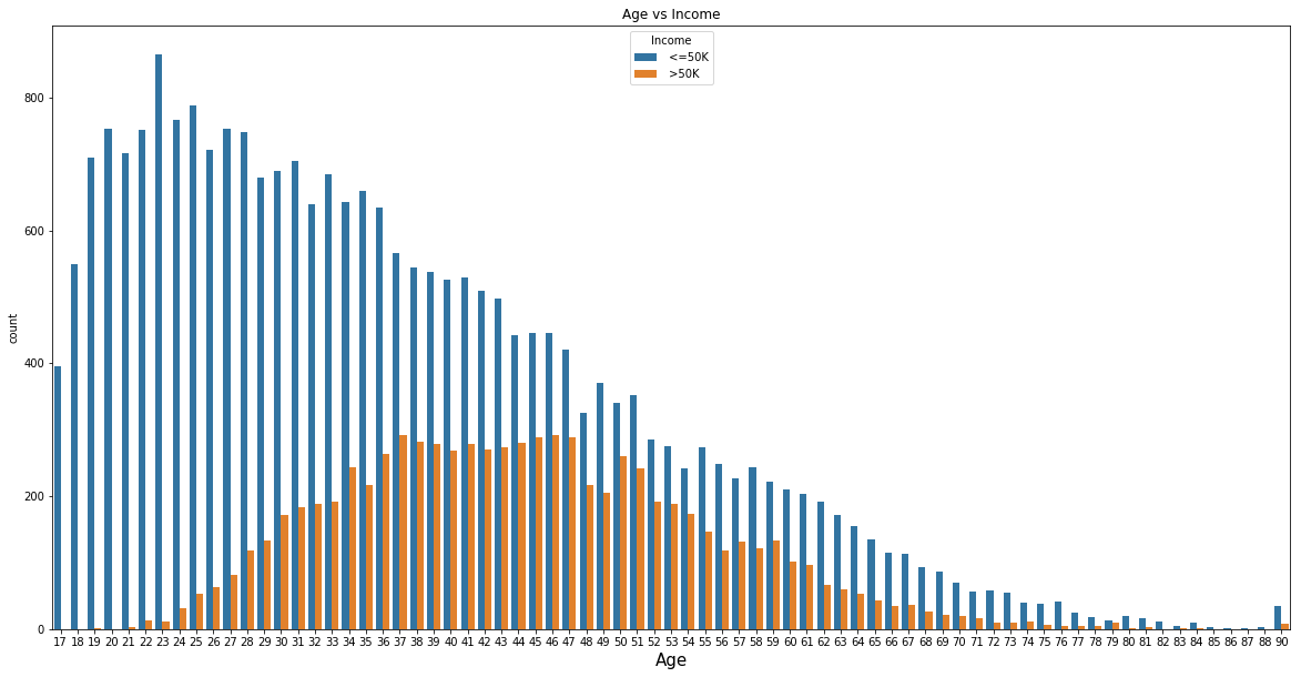
As we might notice seems impossible for people who are less than 20 years old or more than 80 years old to earn more than 50K . At the age of 37 is where we have the most part of people earning 50K. The same occurs at age 46
Race vs Income
plt.figure(figsize=(20,4))
plt.title('Race vs Income')
plt.xlabel('Race', fontsize=15)
sns.countplot(x = 'Race',hue='Income', data=us_adult_income)
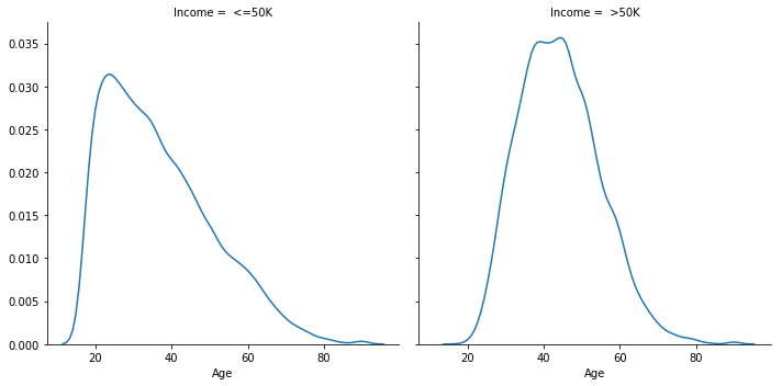
Income Distribution vs Age
density = sns.FacetGrid(us_adult_income, col = "Income",height=5)
density.map(sns.kdeplot, "Age")
Correlation Heat map
fig, (ax) = plt.subplots(1, 1, figsize=(10,6))

hm = sns.heatmap(us_adult_income.corr(),
                 ax=ax,           # Axes in which to draw the plot, otherwise use the currently-active Axes.
                 cmap="coolwarm", # Color Map.
                 #square=True,    # If True, set the Axes aspect to “equal” so each cell will be square-shaped.
                 annot=True,
                 fmt='.2f',       # String formatting code to use when adding annotations.
                 #annot_kws={"size": 14},
                 linewidths=.05)

fig.subplots_adjust(top=0.93)
fig.suptitle('US DATA INCOME Correlation Heatmap',
              fontsize=14,
              fontweight='bold')
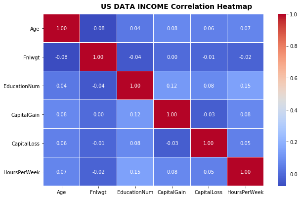
There is not an strong correlation that we can point out but we could mention that Fnlwgt have an inverse correlation to the quantitive variables in the showed in the heat map, except Capital gain.
Since Education Num and Education are the same we are only going to keep the quantitive variable.
del us_adult_income['Education']
Nan Values in our dataset
us_adult_income.isnull().sum()
| Variable | Nan values |
|---|---|
| Age | 0 |
| Workclass | 1836 |
| Fnlwgt | 0 |
| EducationNum | 0 |
| MaritalStatus | 0 |
| Occupation | 1843 |
| Relationship | 0 |
| Race | 0 |
| Gender | 0 |
| CapitalGain | 0 |
| CapitalLoss | 0 |
| HoursPerWeek | 0 |
| Country | 583 |
| Income | 0 |
us_adult_income.Income.value_counts()
| Target | Quantity |
|---|---|
| <=50K | 24720 |
| >50K | 7841 |
Most of our dataset belongs to the class <=50K
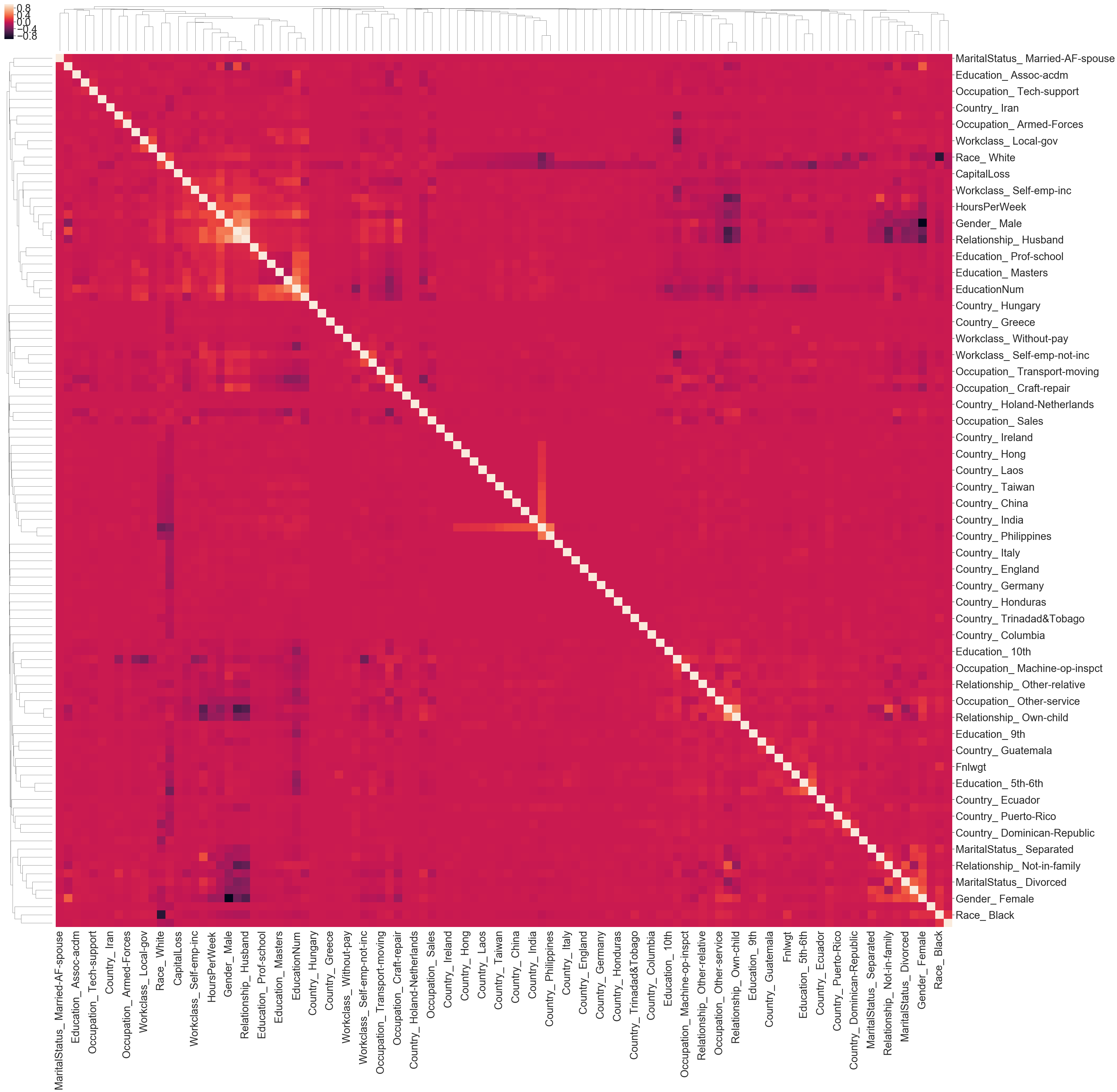
Encoding
We encode the categorical variables in order to train our model. We replace the missing values with the statistical mean of each column.
one_hot_encoding = pd.get_dummies(us_adult_income)
one_hot_encoding.fillna(one_hot_encoding .mean(),inplace=True)
one_hot_encoding["Income"] = one_hot_encoding['Income_ >50K']
del one_hot_encoding['Income_ <=50K']
del one_hot_encoding['Income_ >50K']
sns.set(font_scale=2.8)
sns.clustermap(one_hot_encoding.corr(), metric="correlation",figsize=(50, 50))
Split the dataset into train and testing
X = one_hot_encoding.iloc[:,0:-1]
y = one_hot_encoding.iloc[:,-1]
X_train, X_test, y_train, y_test = train_test_split(X,y, test_size = 0.25, random_state = 42)
Random Forest Classifier
rf = RandomForestClassifier(max_depth=25,n_estimators=200, min_samples_leaf=1,min_samples_split=50,criterion='entropy', oob_score=True,random_state=42)
rf.fit(X_train, y_train)
predicted = rf.predict(X_test)
accuracy = accuracy_score(y_test, predicted)
print(f'Out-of-bag score estimate: {rf.oob_score_:.3}')
print(f'Mean accuracy score: {accuracy:.3}')
Estimation
Out-of-bag score estimate: 0.862
Mean accuracy score: 0.866
Confusion Matrix
cm = confusion_matrix(y_test, predicted)
fig, (ax) = plt.subplots(1, 1, figsize=(8,7))
sns.heatmap(cm, annot=True, ax = ax,fmt='g')
# labels, title and ticks
ax.set_xlabel('Predicted labels')
ax.set_ylabel('True labels');
ax.set_title('Confusion Matrix')
sns.set(font_scale=1.5)
ax.xaxis.set_ticklabels(['Income > 50 K', 'Income < 50 K'])
ax.yaxis.set_ticklabels(['Income > 50 K', 'Income < 50 K'])
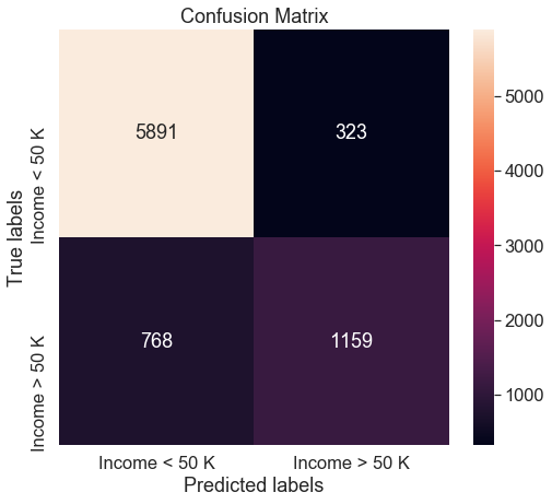
Conclusion
Random forest performs well, maybe if we have more individuals that make more than 50 K, it might be easier for the model to predict those cases. Maybe we could have chosen to remove the column Fnlwgt, which seems not to aport a great deal of information, the same with Capital Gains\Loss and Relationship.